eEvents_df: compute expected number of events at 1 time point

Introduction of `eEvents_df`

eEvents_df() computes expected number of events at a given analysis time by strata under the assumption of piecewise model:

piecewise constant enrollment rates
piecewise exponential failure rates
piecewise censoring rates.

The above piecewise exponential distribution allows a simple method to specify a distribution and enrollment pattern where the enrollment, failure and dropout rates changes over time.

Here the df in eEvents_df() is short for data frame, since its output is a data frame.

Use Cases

Example 1: Single Enroll + Single Fail Period

enrollRates <- tibble(duration = 10, rate = 10)
failRates <- tibble(duration = 100, failRate = log(2) / 6, dropoutRate = .01)
totalDuration <- 22

eEvents_df(enrollRates = enrollRates, failRates = failRates, totalDuration = totalDuration, simple = FALSE)

## # A tibble: 1 × 3
##       t failRate Events
##   <dbl>    <dbl>  <dbl>
## 1     0    0.116   80.4

Example 2: Multiple Enroll + Single Fail Period

enrollRates <- tibble(duration = c(5, 5), rate = c(10, 20))
failRates <- tibble(duration = 100, failRate = log(2)/6, dropoutRate = .01)
totalDuration <- 22

eEvents_df(enrollRates = enrollRates, failRates = failRates, totalDuration = totalDuration, simple = FALSE)

## # A tibble: 1 × 3
##       t failRate Events
##   <dbl>    <dbl>  <dbl>
## 1     0    0.116   119.

Example 3: Signle Enroll + Multiple Fail Period

enrollRates <- tibble(duration = 10, rate = 10)
failRates <- tibble(duration = c(20, 80), failRate = c(log(2)/6, log(2)/4), dropoutRate = .01)
totalDuration <- 22

eEvents_df(enrollRates = enrollRates, failRates = failRates, totalDuration = totalDuration, simple = FALSE)

## # A tibble: 2 × 3
##       t failRate Events
##   <dbl>    <dbl>  <dbl>
## 1     0    0.116 80.2  
## 2    20    0.173  0.250

Example 4: Multiple Duration

enrollRates <- tibble(duration = 10, rate = 10)
failRates <- tibble(duration = 100, failRate = log(2) / 6, dropoutRate = .01)
totalDuration <- c(2, 22)

try(eEvents_df(enrollRates = enrollRates, failRates = failRates, totalDuration = totalDuration, simple = FALSE))

## Error in eEvents_df(enrollRates = enrollRates, failRates = failRates,  : 
##   gsDesign2: totalDuration in `events_df()` must be a numeric number!

Inner Logic of `eEvents_df()`

Step 1: set the analysis time.

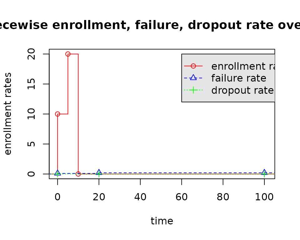
totalDuration <- 50

Step 2: set the enrollment rates.

enrollRates <- tibble(duration = c(5, 5), rate = c(10, 20))

# create a step function (sf) to define enrollment rates over time
sf.enrollRate <- stepfun(c(0, cumsum(enrollRates$duration)),
                         c(0, enrollRates$rate, 0),
                         right = FALSE)

plot(sf.enrollRate, 
     xlab = "duration", ylab = "enrollment rates", 
     main = "Piecewise enrollment rate over time", xlim = c(-0.01, 21))

Step 3: set the failure rates and dropout rates.

failRates <- tibble(duration = c(20, 80), failRate = c(0.1, 0.2), dropoutRate = .01)

# get the time points where the failure rates change
startFail <- c(0, cumsum(failRates$duration))

# plot the piecewise failure rates
sf.failRate <- stepfun(startFail,
                       c(0, failRates$failRate, last(failRates$failRate)),
                       right = FALSE)
plot(sf.failRate, 
     xlab = "duration", ylab = "failure rates", 
     main = "Piecewise failure rate over time", xlim = c(-0.01, 101))

# plot the piecewise dropout rate
sf.dropoutRate <- stepfun(startFail,
                          c(0, failRates$dropoutRate, last(failRates$dropoutRate)),
                          right = FALSE)
plot(sf.dropoutRate, 
     xlab = "duration", ylab = "dropout rates", 
     main = "Piecewise dropout rate over time", xlim = c(-0.01, 101))

Given the above piecewise enrollment rates, failure rates, dropout rates, the time line is divided into several parts:

\((0, 5]\) (5 is the change point of the enrollment rates);
\((5, 10]\) (10 is another change point of the enrollment rates);
\((10, 20]\) (20 is the change point of the failure rates);
\((20, 50]\) (50 is the analysis time);
\((50, \infty]\) (after the analysis time).

Given the above sub-intervals, our objective is to calculate the expected number of events in each sub-intervals.

Step 4: divide the time line for enrollments

df_1 <- tibble(startEnroll = c(0, cumsum(enrollRates$duration)),
               endFail = totalDuration - startEnroll,
               rate = c(enrollRates$rate, 0))

startEnroll¹	endFail²	rate³
df_1
0	50	10
5	45	20
10	40	0
¹ The time when the enrollment starts.
² The time from startEnroll to the analysis time.
³ The enrollment rates

Step 5: divide the time line for failure & dropout rates

df_2 <- tibble(endFail = cumsum(failRates$duration),
               startEnroll = totalDuration - endFail,
               failRate = failRates$failRate,
               dropoutRate = failRates$dropoutRate)

endFail¹	startEnroll²	failRate³	dropoutRate⁴
df_2
20	30	0.1	0.01
100	-50	0.2	0.01
¹ The time when the failure changes.
² The time from endFail to the analysis time.
³ The failure rates
⁴ The dropout rates

For the above df_2, one needs to discriminate if the analysis time (totalDuration = 50) is beyond the total failure rate duration.

# if the analysis time is after the total failure rate duration
if(sum(failRates$duration) < totalDuration){
  df_2 <- df_2[-nrow(df_2), ]
}else{
  df_2 <- df_2 %>% filter(startEnroll > 0)
}

endFail¹	startEnroll²	failRate³	dropoutRate⁴
df_2
Updated by adjusting the analysis time and failRates duration
20	30	0.1	0.01
¹ The time when the failure changes.
² The time from endFail to the analysis time.
³ The failure rates
⁴ The dropout rates

Step 6: divide the time line considering both the change points in enrollment, failure, dropout rates.

df <- full_join(df_1, df_2, by = c("startEnroll", "endFail")) %>% arrange(endFail)

startEnroll¹	endFail²	rate³	failRate	dropoutRate
df
30	20	NA	0.1	0.01
10	40	0	NA	NA
5	45	20	NA	NA
0	50	10	NA	NA
¹ The time when the enrollment rate starts.
² The time when the failure rate ends. And startEnroll + endFail = 50
³ The enrollment rates.

We find there are lots of NA, which can be imputed by the piecewise model.

df <- df %>% mutate(endEnroll = lag(startEnroll, default = as.numeric(totalDuration)),
                    startFail = lag(endFail, default = 0),
                    duration = endEnroll - startEnroll,
                    failRate = sf.failRate(startFail),
                    dropoutRate = sf.dropoutRate(startFail),
                    enrollRate = sf.enrollRate(startEnroll)) %>% 
             select(-rate)

startEnroll¹	endEnroll²	startFail³	endFail⁴	enrollRate	failRate	dropoutRate	duration⁵
0	5	45	50	10	0.2	0.01	5
5	10	40	45	20	0.2	0.01	5
10	30	20	40	0	0.2	0.01	20
30	50	0	20	0	0.1	0.01	20
¹ The time when the enrollment rate starts.
² The (startEnroll, endEnroll] forms the piecewise model of the enrollment rates
³ The time when the failure rate starts.
⁴ The time when the failure rate ends. And startEnroll + endFail = 50. Besides, (startFail, endFail ] forms the piecewise model of the enrollment rates.
⁵ endEnroll - startEnroll

Step 7: compute the expected number of events in sub-intervals following the technical details in the vignette ``computing expected events by interval at risk’’

             # create 2 auxiliary variable for failure & dropout rate
             # q: number of expected events in a sub-interval
             # Q: cumulative product of q (pool all sub-intervals)
df <- df %>% mutate(q = exp(-duration * (failRate + dropoutRate)),
                    Q = lag(cumprod(q), default = 1)) %>%
             arrange(desc(startFail)) %>%
             # create another 2 auxiliary variable for enroll rate
             # g: number of expected subjects in a sub-interval
             # G: cumulative sum of g (pool all sub-intervals)
             mutate(g = enrollRate * duration,
                    G = lag(cumsum(g), default = 0)) %>%
             arrange(startFail) %>%
             # compute expected events as nbar in a sub-interval
             mutate(d = ifelse(failRate == 0, 0, Q * (1 - q) * failRate / (failRate + dropoutRate)),
                    nbar = ifelse(failRate == 0, 0, G * d + (failRate * Q * enrollRate) / (failRate + dropoutRate) * (duration - (1 - q) / (failRate + dropoutRate))))

Step 8: output results

sf.startFail <- stepfun(startFail, c(0, startFail), right = FALSE)
df <- df %>% 
  transmute(t = endFail, failRate = failRate, Events = nbar, startFail = sf.startFail(startFail)) %>% 
  group_by(startFail) %>%
  summarize(failRate = first(failRate), Events = sum(Events)) %>%
  mutate(t = startFail) %>% 
  select("t", "failRate", "Events")

df %>% gt()

t	failRate	Events
0	0.1	121.25411
20	0.2	15.71391

Introduction of eEvents_df