Futility bounds at design and analysis under non-proportional hazards • gsDesign2

library(gsDesign2)
library(gt)
library(dplyr)
library(tibble)
library(ggplot2)

Overview

We set up futility bounds under a non-proportional hazards assumption. We consider methods presented by Korn and Freidlin (2018) for setting such bounds and then consider an alternate futility bound based on \(\beta\)-spending under a delayed or crossing treatment effect to simplify implementation. Finally, we show how to update this \(\beta\)-spending bound based on blinded interim data. We will consider an example to reproduce a line of Korn and Freidlin (2018) Table 1 with the alternative futility bounds considered.

Initial design set-up for fixed analysis

Korn and Freidlin (2018) considered delayed effect scenarios and proposed a futility bound that is a modification of an earlier method proposed by Wieand, Schroeder, and O’Fallon (1994). We begin with the enrollment and failure rate assumptions which Korn and Freidlin (2018) based on an example by Chen (2013).

# Enrollment assumed to be 680 patients over 12 months with no ramp-up
enrollRates <- tibble(Stratum = "All", duration = 12, rate = 680 / 12)
# Failure rates
## Control exponential with median of 12 mos
## Delayed effect with HR = 1 for 3 months and HR = .693 thereafter
## Censoring rate is 0
failRates <- tibble(Stratum = "All", duration = c(3, 100), 
                   failRate = -log(.5) / 12, hr = c(1, .693), dropoutRate = 0)
## Study duration was 34.8 in Korn & Freidlin Table 1
## We change to 34.86 here to obtain 512 expected events more precisely
studyDuration <- 34.86

We now derive a fixed sample size based on these assumptions. Ideally, we would allow a targeted event count and variable follow-up in fixed_design() so that the study duration will be computed automatically.

fixedevents <- fixed_design(x = "AHR", alpha = 0.025, power = NULL, 
                      enrollRates = enrollRates,
                      failRates = failRates,
                      studyDuration = studyDuration)
fixedevents %>% summary() %>% 
  select(-Bound) %>%
  as_gt(footnote="Power based on 512 events") %>%
  fmt_number(columns = 3:4, decimals = 2) %>% 
  fmt_number(columns = 5:6, decimals = 3)

Design	N	Events	Time	alpha	Power
Fixed Design under AHR Method¹
AHR	680	511.99	34.86	0.025	0.905
¹ Power based on 512 events

Modified Wieand futility bound

The Wieand, Schroeder, and O’Fallon (1994) rule recommends stopping after 50% of planned events accrue if the observed HR > 1. Korn and Freidlin (2018) modified this by adding a second interim analysis after 75% of planned events and stop if the observed HR > 1 This is implemented here by requiring a trend in favor of control with a direction \(Z\)-bound at 0 resulting in the Nominal p bound being 0.5 for interim analyses in the table below. A fixed bound is specified with the gs_b() function for upper and lower and corresponding parameters upar for the upper (efficacy) bound and lpar for the lower (futility) bound. The final efficacy bound is for a 1-sided nominal p-value of 0.025; the futility bound lowers this to 0.0247 as noted in the lower-right-hand corner of the table below. In the last row under Alternate hypothesis below we see the power is 88.44%. Korn and Freidlin (2018) computed 88.4% power for this design with 100,000 simulations which estimate the standard error for the power calculation to be 0.1%.

wieand <- gs_power_ahr(enrollRates = enrollRates, failRates = failRates,
                       upper = gs_b, upar = c(rep(Inf, 2), qnorm(.975)),
                       lower = gs_b, lpar = c(0, 0, -Inf),
                       events = 512 * c(.5, .75, 1))
wieand %>% summary() %>% 
  as_gt(title="Group sequential design with futility only at interim analyses",
        subtitle="Wieand futility rule stops if HR > 1")

Bound	Nominal p¹	~HR at bound²	Cumulative boundary crossing probability
Group sequential design with futility only at interim analyses
Wieand futility rule stops if HR > 1
Bound	Nominal p¹	~HR at bound²	Alternate hypothesis	Null hypothesis
Analysis: 1 Time: 15.4 N: 680 Events: 256 AHR: 0.81 IF: 0.5
Futility	0.500	1.0000	0.0462	0.5000
Efficacy	0.000	0.0000	0.0000	0.0000
Analysis: 2 Time: 22.9 N: 680 Events: 384 AHR: 0.77 IF: 0.75
Futility	0.500	1.0000	0.0469	0.5980
Efficacy	0.000	0.0000	0.0000	0.0000
Analysis: 3 Time: 34.9 N: 680 Events: 512 AHR: 0.75 IF: 1
Futility	1.000	Inf	0.0469	0.5980
Efficacy	0.025	0.8405	0.8844	0.0247
¹ One-sided p-value for experimental vs control treatment. Values < 0.5 favor experimental, > 0.5 favor control.
² Approximate hazard ratio to cross bound.

Beta-spending futility bound with AHR

Need to summarize here.

betaspending <- gs_power_ahr(enrollRates = enrollRates, failRates = failRates,
                       upper = gs_b, upar = c(rep(Inf, 2), qnorm(.975)),
                       lower = gs_spending_bound, 
                       lpar = list(sf = gsDesign::sfLDOF, total_spend = 0.025,
                                   param = NULL, timing = NULL),
                       events = 512 * c(.5, .75, 1),
                       test_lower = c(TRUE, TRUE, FALSE))
betaspending %>% 
  summary() %>% as_gt(title="Group sequential design with futility only",
                      subtitle="Beta-spending futility bound")

Bound	Nominal p¹	~HR at bound²	Cumulative boundary crossing probability
Group sequential design with futility only
Beta-spending futility bound
Bound	Nominal p¹	~HR at bound²	Alternate hypothesis	Null hypothesis
Analysis: 1 Time: 15.4 N: 680 Events: 256 AHR: 0.81 IF: 0.5
Futility	0.9015	1.1762	0.0015	0.0015
Efficacy	0.0000	0.0000	0.0000	0.0000
Analysis: 2 Time: 22.9 N: 680 Events: 384 AHR: 0.77 IF: 0.75
Futility	0.4206	0.9796	0.0095	0.0096
Efficacy	0.0000	0.0000	0.0000	0.0000
Analysis: 3 Time: 34.9 N: 680 Events: 512 AHR: 0.75 IF: 1
Futility	1.0000	Inf	0.0095	0.0096
Efficacy	0.0250	0.8405	0.9031	0.0250
¹ One-sided p-value for experimental vs control treatment. Values < 0.5 favor experimental, > 0.5 favor control.
² Approximate hazard ratio to cross bound.

Classical beta-spending futility bound

A classical \(\beta\)-spending bound would assume a constant treatment effect over time using the proportional hazards assumption. We use the average hazard ratio at the fixed design analysis for this purpose.

Korn and Freidlin futility bound

The Korn and Freidlin (2018) futility bound is set when at least 50% of the expected events have occurred and at least two thirds of the observed events have occurred later than 3 months from randomization. The expected timing for this is demonstrated below.

Accumulation of events by time interval

We consider the accumulation of events over time that occur during the no-effect interval for the first 3 months after randomization and events after this time interval. This is done for the overall trial without dividing out by treatment group using the gsDesign2::AHR() function. We consider monthly accumulation of events through the 34.86 months planned trial duration. We note in the summary of early expected events below that all events during the first 3 months on-study are expected prior to the first interim analysis.

event_accumulation <- 
AHR(enrollRates = enrollRates,
    failRates = failRates,
    totalDuration = c(1:34, 34.86),
    ratio = 1,
    simple = FALSE)
head(event_accumulation, n = 7) %>% gt()

Time	Stratum	t	HR	Events	info	info0
1	All	0	1.000	1.605536	0.4013840	0.4013840
2	All	0	1.000	6.301416	1.5753540	1.5753540
3	All	0	1.000	13.914192	3.4785480	3.4785480
4	All	0	1.000	22.930062	5.7325155	5.7325155
4	All	3	0.693	1.145602	0.2772752	0.2864004
5	All	0	1.000	31.945932	7.9864829	7.9864829
5	All	3	0.693	4.506946	1.0919515	1.1267364

We can look at the proportion of events after the first 3 months as follows:

event_accumulation %>% 
  group_by(Time) %>%
  summarize(`Total events` = sum(Events), "Proportion early" = first(Events) /  `Total events`) %>%
  ggplot(aes(x=Time, y=`Proportion early`)) + geom_line()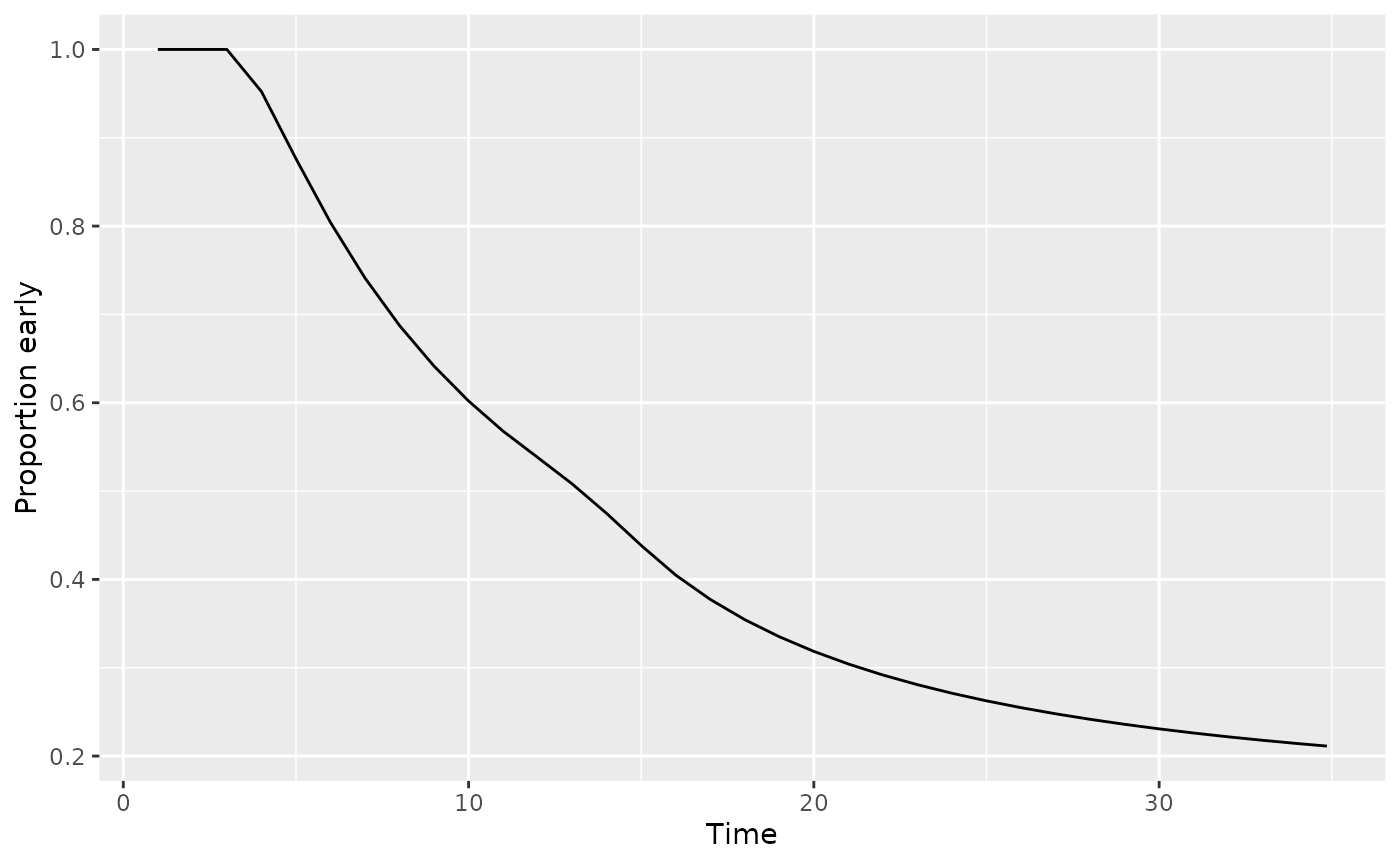

For the Korn and Freidlin (2018) bound the targeted timing is when both 50% of events have occurred and at least 2/3 are more than 3 months after enrollment with 3 months being the delayed effect period. We see above that about 1/3 of events are still within 3 months of enrollment at month 20.

Korn and Freidlin bound

The bound proposed by Korn and Freidlin (2018)

Updating beta=spending bound at time of analysis

We provide an example of how to update a \(\beta\)-spending bound using blinded data when a piecewise constant hazard ratio is assumed. The basic approach is as follows:

For each piecewise interval in the design with a different hazard ratio, compute the blinded total events and total follow-up time.
Compute variance and statistical information under the null hypothesis for each interval in the piecewise model. This assumes equal censoring in the two arms. Assuming equal randomization and equal dropout rates in the two arms.

References

Chen, Tai-Tsang. 2013. “Statistical Issues and Challenges in Immuno-Oncology.” Journal for Immunotherapy of Cancer 1 (1): 1–9.

Korn, Edward L, and Boris Freidlin. 2018. “Interim Futility Monitoring Assessing Immune Therapies with a Potentially Delayed Treatment Effect.” Journal of Clinical Oncology 36 (23): 2444.

Wieand, Sam, Georgene Schroeder, and Judith Rich O’Fallon. 1994. “Stopping When the Experimental Regimen Does Not Appear to Help.” Statistics in Medicine 13 (13-14): 1453–8.